ICON in single-column and large-eddy simulation mode#
ICON’s single-column model (SCM) and large-eddy simulation (LES) capabilities provide a framework for detailed atmospheric process studies and turbulence-resolving simulations. As described by Ďurán et al. (2021), ICON-SCM is implemented internally within the main ICON model code - not as an external driver or wrapper like many other modeling systems. By setting ldynamics=.false. in the namelist, the full 3D model collapses to column mode, ensuring that SCM configurations use identical physics parameterizations and numerical schemes as operational forecasts and climate simulations.
ICON-SCM and ICON-LES share the same grid infrastructure, differing only in domain size: SCM uses minimal torus grids (4×4×2 triangular cells) where all columns experience identical forcing, while LES employs larger domains with periodic boundaries to resolve turbulent eddies explicitly.
Reference: Ďurán, I., Köhler, M., Eichhorn-Müller, A., Maurer, V., Schmidli, J., Schomburg, A., et al. (2021). The ICON single-column mode. Atmosphere, 12, 906. doi:10.3390/atmos12070906
Concept and Design#
ICON-SCM and ICON-LES operate on torus grids - doubly-periodic domains with triangular cells. The torus geometry is activated by setting is_plane_torus=.TRUE. in the grid namelist, which establishes periodic boundary conditions in both horizontal directions.
The distinction between SCM and LES modes lies in the treatment of dynamics and transport:
SCM mode: Dynamics and transport are disabled (
ldynamics=.FALSE.,ltransport=.FALSE.). All grid cells experience identical forcing and evolve identically. The minimal 4×4×2 triangular cell grid is sufficient since no horizontal interactions occur.LES mode: Dynamics and transport are enabled (
ldynamics=.TRUE.,ltransport=.TRUE.). Turbulent eddies develop and interact horizontally. Typical LES grids use 100×100 cells at 100 m resolution to adequately resolve the turbulent cascade.
Switching between SCM and LES requires changing only two namelist parameters (ldynamics and ltransport), making it straightforward to test physics schemes in idealized single-column mode before evaluating their behavior in turbulence-resolving simulations.
Both modes share identical physics parameterizations with operational ICON, differing only in physics scheme selection (e.g., TKE turbulence vs Smagorinsky LES, convection on/off) and grid configuration. This internal implementation ensures consistency across all ICON applications without code duplication.
Workflow#
ICON-SCM/LES simulations follow a three-stage workflow organized in the scripts/scm directory:
1. Initial condition creation (scripts/scm/init_create/)
Initial conditions can be generated from two sources:
From 3D ICON runs: Extract profiles for a specific location and time using
get_SCM_data_ICON.py:python3 get_SCM_data_ICON.py <lat> <lon> <inidate> python3 get_SCM_data_ICON.py 52.2 14.1 2020112400
This workflow requires running ICON with the
run_ICON_4_SCMiniscript to prepare forcing data, then extracting profiles and creating external parameters withcreate_SCM_extpar_ICON.py.From DEPHY idealized cases: Standardized forcing files in DEPHY format are available for canonical test cases (ARM, BOMEX, RICO, GABLS1, FIRE, MPACE, MAGIC, COMBLE, CP-MIP). Case-specific scripts (e.g.,
get_ARM_data.py,get_BOMEX_data.py) generate these forcing files.
2. Model execution (scripts/scm/run/)
Run scripts configure and execute ICON-SCM or ICON-LES. For DEPHY cases, use the unified scripts:
run_SCM_dephycases_nec- SCM mode for all DEPHY casesrun_LES_dephycases_nec- LES mode for all DEPHY cases
Set the desired case via CASE=ARM (or RICO, BOMEX, etc.) in the script. Case-specific parameters (Coriolis latitude, surface boundary conditions, forcing options) are loaded from case_definition_dephy.s.
3. Visualization (scripts/scm/plot/)
Analysis scripts produce various diagnostics:
plot-scm-time-z.py- Time-height cross-sectionsplot-scm-var-z.py- Vertical profilesplot-scm-time-var.py- Time seriesplot-scm+les-*.py- Combined SCM/LES comparisonsplot-all.py- Batch processing for multiple variables/cases
Initial and Forcing Conditions#
Initial conditions and large-scale forcing can be provided from idealized case studies or generated by archiving forcing for a single grid cell from a full 3D ICON run (see Workflow above, use namelist setting i_scm_netcdf=1 in scm_nml)
DEPHY Format#
The preferred format for forcing files is the DEPHY SCM format (https://github.com/GdR-DEPHY/DEPHY-SCM), which provides standardized input for intercomparison studies. ICON supports DEPHY format via the namelist setting i_scm_netcdf=2 in scm_nml. A collection of canonical cases is available locally on the DWD RCL system.
Available Test Cases#
The following DEPHY cases are configured in case_definition_dephy.s:
Case |
Duration |
Location |
Description |
|---|---|---|---|
ARM |
14.5 h |
35.0°N |
Continental shallow cumulus |
RICO |
24 h |
18.0°N |
Trade wind cumulus |
BOMEX |
24 h |
14.94°N |
Marine stratocumulus-to-cumulus |
GABLS1 |
9 h |
73.0°N |
Stable boundary layer (dry) |
FIRE |
37 h |
33.3°N |
Stratocumulus-topped boundary layer |
MPACE |
13 h |
71.75°N |
Mixed-phase Arctic clouds |
MAGIC |
106 h |
NE Pacific |
Marine stratocumulus-to-cumulus |
COMBLE |
37 h |
74.5°N |
Cold-air outbreak |
CP-MIP |
34 h |
N Atlantic |
Marine cold pool case from EUREC4A |
Forcing Options#
Large-scale forcing is configured via the ls_forcing_nml namelist. Available forcing terms include:
Geostrophic wind forcing (
is_geowind=.TRUE.) - applies pressure gradient force when geostrophic winds are provided in the forcing fileSubsidence - vertical advection for momentum (
is_subsidence_moment=.TRUE.) and thermodynamic variables (is_subsidence_heat=.TRUE.)Horizontal advection - tendencies from large-scale flow (
is_advection=.TRUE.), with separate switches for winds (is_advection_uv) and thermodynamic variables (is_advection_tq)Radiative forcing - prescribed radiative heating rates (
is_rad_forcing=.TRUE.)
Coriolis Forcing#
The Coriolis forcing can be applied in two ways: as part of the large-scale forcing using domain-average horizontal winds (is_ls_coriolis=.TRUE.), or by letting the dynamics calculate this term (lcoriolis=.TRUE.). The second option is only available in LES mode where dynamic transport occurs. For SCM mode, the first option must be selected. The two options are mutually exclusive, and is_ls_coriolis will be set to .FALSE. with a warning message if both are selected.
Grids and Running#
Torus Grids#
Both SCM and LES modes run on torus grids with doubly-periodic boundary conditions. Pre-generated grids are available on the DWD RCL system at /hpc/uwork/mkoehler/scm/data/grid/:
Grid File |
Configuration |
Typical Use |
|---|---|---|
Torus_Triangles_4x4_2500m.nc |
4×4 cells, 2.5 km |
SCM |
Torus_Triangles_50x50_200m.nc |
50×50 cells, 200 m |
LES |
Torus_Triangles_100x100_100m.nc |
100×100 cells, 100 m |
LES |
Torus_Triangles_200x200_1250m.nc |
200×200 cells, 1.25 km |
CRM |
Additional torus grids can be generated with the grid generator developed by Leonidas Linardakis at MPI-Meteorology.
In SCM mode, each grid point experiences identical forcing with no horizontal interactions, making the minimal 4×4 grid sufficient. For LES simulations, larger domains are required to adequately resolve turbulent eddies.
Run Scripts#
Sample run scripts for the DWD RCL system are provided in scripts/scm/run/. The unified scripts for DEPHY cases are:
run_SCM_dephycases_nec- SCM mode for all DEPHY test casesrun_LES_dephycases_nec- LES mode for all DEPHY test cases
To run a specific case, edit the script and set CASE=ARM (or RICO, BOMEX, GABLS1, FIRE, MPACE, MAGIC, COMBLE). Case-specific parameters including Coriolis latitude, surface boundary conditions, and forcing options are automatically loaded from case_definition_dephy.s.
For runs using ICON initial conditions:
run_SCM_ICONini- SCM with ICON forcingrun_LES_ICONini- LES with ICON forcing
Additional case-specific scripts (e.g., run_SCM_ARM, run_SCM_BOMEX) are available for individual test cases.
Namelist Configuration#
Basic Mode Selection#
The fundamental difference between SCM and LES modes is controlled by switches in run_nml and grid_nml:
grid_nml:
&grid_nml
  dynamics_grid_filename = "Torus_Triangles_4x4_2500m.nc"
  is_plane_torus         = .TRUE.    ! Doubly-periodic torus grid
  l_scm_mode             = .TRUE.    ! Master switch for SCM mode
  corio_lat              = 35.0      ! Coriolis latitude [degrees]
/
run_nml:
Parameter |
SCM Mode |
LES Mode |
Description |
|---|---|---|---|
|
|
|
Compute adiabatic dynamics |
|
|
|
Tracer transport |
|
|
|
Enable test case mode |
Large-Scale Forcing#
Configure forcing terms in ls_forcing_nml:
&ls_forcing_nml
  is_geowind           = .TRUE.    ! Apply geostrophic wind forcing
  is_subsidence_moment = .FALSE.   ! Subsidence for u,v
  is_subsidence_heat   = .TRUE.    ! Subsidence for T,q
  is_advection         = .TRUE.    ! Horizontal advection forcing
  is_advection_uv      = .TRUE.    ! Advection for u,v
  is_advection_tq      = .TRUE.    ! Advection for T,q
  is_rad_forcing       = .FALSE.   ! Radiative forcing
/
The Coriolis forcing can be applied via large-scale forcing using domain-average winds (is_ls_coriolis=.TRUE.) or through the dynamics (lcoriolis=.TRUE. in dynamics_nml). The dynamics option is only available in LES mode. These options are mutually exclusive.
Nudging Configuration#
The SCM/LES can be nudged towards background profiles for horizontal winds, temperature, and humidity. Each variable has separate relaxation timescales and height specifications:
&ls_forcing_nml
  is_nudging            = .TRUE.     ! Master nudging switch
  is_nudging_uv         = .TRUE.     ! Nudge winds
  is_nudging_t          = .TRUE.     ! Nudge temperature
  is_nudging_q          = .TRUE.     ! Nudge moisture

  ! Nudging heights and timescales
  nudge_start_height_uv = 2000.0     ! UV nudging starts [m]
  nudge_full_height_uv  = 3000.0     ! UV nudging full strength [m]
  dt_relax_uv           = 3600.0     ! UV relaxation timescale [s]

  nudge_start_height_t  = 2000.0     ! T nudging starts [m]
  nudge_full_height_t   = 3000.0     ! T nudging full strength [m]
  dt_relax_t            = 3600.0     ! T relaxation timescale [s]

  nudge_start_height_q  = 2000.0     ! q nudging starts [m]
  nudge_full_height_q   = 3000.0     ! q nudging full strength [m]
  dt_relax_q            = 3600.0     ! q relaxation timescale [s]
/
Nudging with full strength is applied above nudge_full_height_*. If a nudge_start_height_* is specified with a lower value, nudging is linearly scaled between the start and full heights, with no nudging below the start height.
SCM-Specific Settings#
Configure input format and boundary conditions in scm_nml:
&scm_nml
  i_scm_netcdf      = 2        ! 0=ASCII, 1=netCDF, 2=DEPHY
  lscm_read_tke     = .FALSE.  ! Read initial TKE
  lscm_read_z0      = .FALSE.  ! Read z0 from netCDF
  lscm_random_noise = .FALSE.  ! Add random noise (for LES)
  scm_sfc_mom       = 0        ! Surface momentum BC: 0=TURBTRANS, 2=u*, 5=MO
  scm_sfc_temp      = 0        ! Surface temp BC: 0=TERRA, 1=Tg, 2=shfl_s
  scm_sfc_qv        = 0        ! Surface moisture BC: 0=TERRA, 1=qv_s, 2=lhfl_s, 3=qv_sat
/
LES-Specific Settings#
Configure turbulence and surface fluxes in les_nml:
&les_nml
  isrfc_type    = 10      ! 1=fixed SST, 2=fixed flux, 3=fixed buoyancy, 10=SCM-like
  sst           = 300.0   ! Prescribed SST [K]
  shflx         = 0.1     ! Sensible heat flux [K m/s]
  lhflx         = 0.0     ! Latent heat flux [K m/s]
  smag_constant = 0.23    ! Smagorinsky constant
  turb_prandtl  = 0.333   ! Turbulent Prandtl number
/
For LES initialization, random perturbations can trigger turbulence development:
&nh_testcases_nml
  w_perturb  = 0.1    ! Random w perturbation [m/s]
  th_perturb = 0.2    ! Random theta perturbation [K]
/
Visualization#
Analysis and plotting scripts are provided in scripts/scm/plot/. These Python scripts read ICON output and produce standard diagnostics for SCM/LES evaluation.
Available Plotting Scripts#
Single-mode diagnostics:
plot-scm-time-z.py- Time-height cross-sections (Hovmöller diagrams)plot-scm-var-z.py- Vertical profiles at specified timesplot-scm-time-var.py- Time series of surface or column-integrated variables
Multi-mode comparisons:
plot-scm+les-time-z.py- SCM and LES time-height comparisonplot-scm+les-var-z.py- SCM and LES vertical profile comparisonplot-scm+les-time-var.py- SCM and LES time series comparison
Specialized tools:
plot-scm+meteogram-*.py- Compare SCM output with operational meteogramsanimated-gif-les.py- Create animations from LES outputplot-all.py- Batch processing for multiple cases and variables
Output Conversion#
ICON output can be converted to DEPHY format for standardized intercomparison using convert_ICONout2dephyV0.s.
Summary#
ICON’s internal SCM and LES capabilities provide a unified framework for atmospheric process studies across scales. The shared codebase ensures consistency between idealized column studies and turbulence-resolving simulations, while the simple two-parameter switch between modes facilitates systematic testing of parameterizations. With standardized DEPHY forcing files and comprehensive analysis tools, ICON-SCM/LES supports educational and research applications as well as model development.
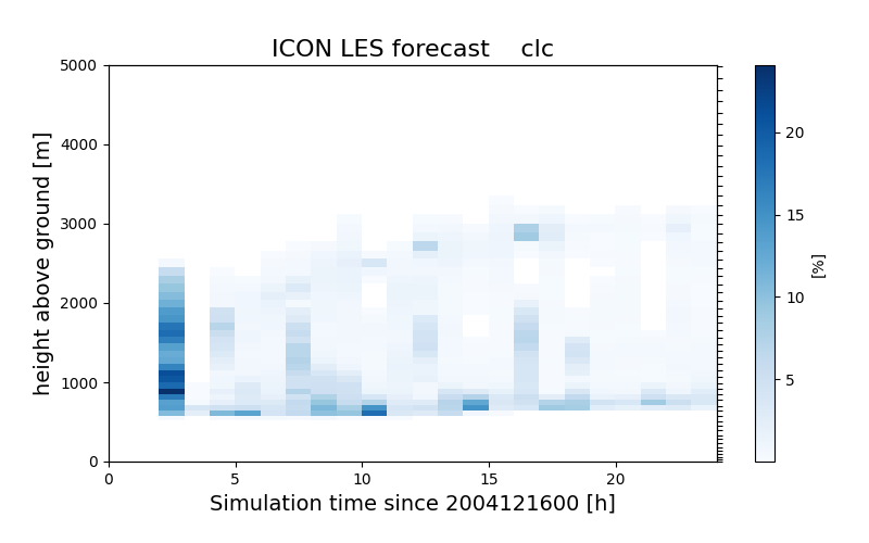
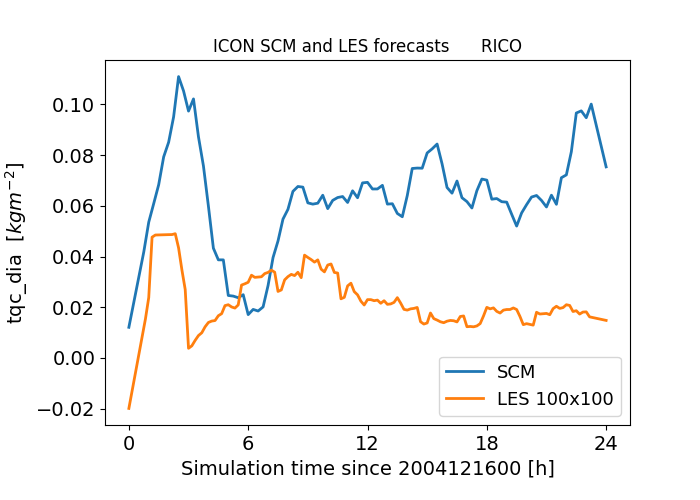
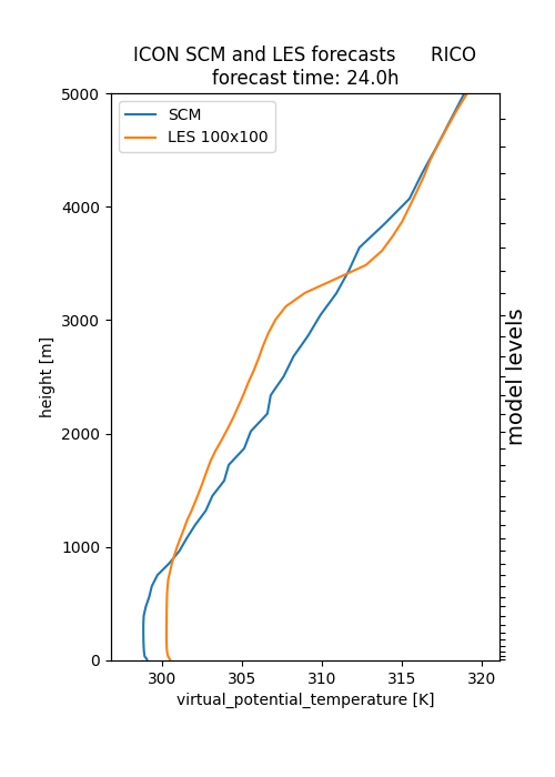
Figure 1: Example ICON-SCM and ICON-LES output for the RICO trade wind cumulus case. Left: Time-height cross-section of cloud cover from LES showing the diurnal evolution of shallow convection. Center: Comparison of domain-mean cloud liquid water path between SCM (blue) and LES (orange), illustrating differences in parameterized versus resolved convection. Right: Vertical profiles of virtual potential temperature at 24h forecast time, showing close agreement in boundary layer structure between SCM and LES modes.