Topographic corrections on surface radiation

In mountainous terrain, the surface energy balance is affected by local and neighbouring terrain in various ways, e. g., modulation of direct-beam shortwave radiation by locally sloped terrain (slope effect) and shadow casting from nearby mountains (topographic/orographic shading). In ICON, all grid cells at the surface are aligned tangentially to the assumed spherical shape of the Earth (i.e., horizontal) and the two-stream approximation solved in the radiation scheme only considers vertical radiative fluxes. Thus the above-mentioned topographic effects on surface radiation must be parameterised (namelist parameter islope_rad). Accounting for these effects in kilometer-scale grid spacing (and below) has significant effects on surface radiation fluxes and linked (near-) surface variables like snow cover and 2 m air temperature and helps to reduce biases in these quantities.

Correction of the direct beam shortwave radiation

To correct the direct beam shortwave radiation for the slope effect and topographic shading, the Sun’s position must be known, which is computed for the present-epoch orbital configuration, following Spencer 1971, i.e., equations (3) and (4)

(1)\[\eta = 0.681 + 0.2422 \, \left(t_{year} - 1949\right) - \left\lfloor \frac{t_{year} - 1949}{4} \right\rfloor\]

(2)\[\beta = \frac{2 \pi \, (t_{doy} - 1 + \eta )}{365.2422}\]

(3)\[e_{time} = 0.000075 + 0.001868 \cos{\beta} - 0.032077 \sin{\beta} - 0.014615 \cos(2 \beta) - 0.040849 \sin(2 \beta)\]

(4)\[\begin{split}\delta = 0.006918 - 0.399912 \cos{\beta} + 0.070257 \sin{\beta} - 0.006758 \cos(2 \beta) \\ + 0.000907 \sin(2 \beta) - 0.002697 \cos(3 \beta) + 0.001480 \sin(3 \beta)\end{split}\]

with \(t_{year}\) representing the year (in the Gregorian calendar), \(t_{doy}\) the day of year, \(\beta\) the fractional year (i.e., the position of Earth in its orbit expressed as a fraction of the orbital period), \(e_{time}\) [rad] the equation of time and \(\delta\) [rad] the Sun’s declination angle measured in an equatorial coordinate system. The denominator in Eq. (2) refers to the number of days in a tropical year.

The angle between the Sun’s position and the prime meridian (Greenwich hour angle) \(\omega_{GHA}\) [rad] is defined as positive west of the meridian plane, and can be computed as

(5)\[\omega_{GHA} = \pi \frac{t_{h} - 12}{12} + e_{time}\]

with \(t_{h}\) representing decimal hours. The latitude and longitude of the subsolar point are thus given by \(\phi_{s} = \delta\) and \(\lambda_{s} = -\omega_{GHA}\), respectively, describing the position of the sun in spherical coordinates in an Earth-centred, Earth-fixed (ECEF) coordinate system:

(6)\[\begin{split}\vec{s}_{ECEF}= \left(\begin{array}{c} \cos{\phi_{s}} \cos{\lambda_{s}} \\ \cos{\phi_{s}} \sin{\lambda_{s}} \\ \sin{\phi_{s}} \end{array}\right)\end{split}\]

Ultimately, the unit Sun position vector is required in a local tangent plane coordinate system (East-North-Up; ENU). The transformation is performed with the following rotation matrix

(7)\[\begin{split}R_{ECEF \rightarrow ENU} = \begin{pmatrix} -\sin{\lambda_{o}} & \cos{\lambda_{o}} & 0 \\ -\sin{\phi_{o}} \cos{\lambda_{o}} & -\sin{\phi_{o}} \sin{\lambda_{o}} & \cos{\phi_{o}} \\ \cos{\phi_{o}} \cos{\lambda_{o}} & \cos{\phi_{o}} \sin{\lambda_{o}} & \sin{\phi_{o}} \end{pmatrix}\end{split}\]

where (\(\phi_{o}\), \(\lambda_{o}\)) represent the latitude and longitude of the ENU coordinate system’s origin. Multiplying Eq. (7) with Eq. (6) yields

(8)\[\begin{split}\vec{s}_{ENU}= \left(\begin{array}{c} \cos{\phi_{s}} \sin{\lambda_{\Delta}} \\ \cos{\phi_{o}} \sin{\phi_s} - \sin{\phi_{o}} \cos{\phi_{s}} \cos{\lambda_{\Delta}} \\ \sin{\phi_{o}} \sin{\phi_s} + \cos{\phi_{o}} \cos{\phi_{s}} \cos{\lambda_{\Delta}} \end{array}\right)\end{split}\]

with \(\lambda_{\Delta} = \lambda_{s} - \lambda_{o}\). Following Zhang 2021, we ignore the positional shift of an object when viewed from two different vantage points (the parallax effect).

To compute the slope effect factor for the direct beam shortwave radiation, two additional unit vectors in the ENU coordinate system have to be defined, namely the normal unit vector of the horizontal surface \(\vec{h}\)

(9)\[\begin{split}\vec{h}_{ENU} = \left(\begin{array}{c} 0 \\ 0 \\ 1 \end{array}\right)\end{split}\]

and the normal unit vector of the locally sloped terrain \(\vec{t}\)

(10)\[\begin{split}\vec{t}_{ENU} = \left(\begin{array}{c} \sin{\theta_{t}} \sin{\gamma_{t}} \\ \sin{\theta_{t}} \cos{\gamma_{t}} \\ \cos{\theta_{t}} \end{array}\right)\end{split}\]

with \(\theta_{t}\) [rad] representing the slope angle and \(\gamma_{t}\) [rad] the aspect angle measured clockwise from North. These two variables are computed within ICON itself from the model topography, which is potentially filtered (i.e., smoothed) during model initialization.

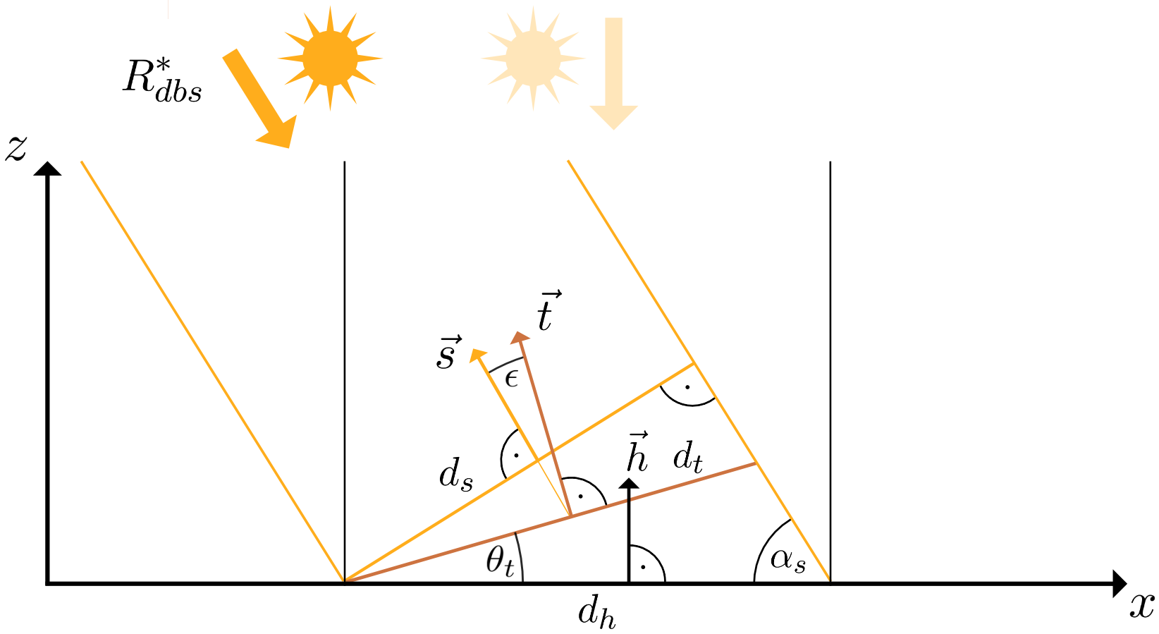
Derivation of the slope effect factor. \(R_{dbs}^*\) represents the direct beam shortwave radiant flux, \(\alpha_{s}\) the solar elevation angle and \(\theta_{t}\) the terrain slope angle. The three unit vectors \(\vec{h}\), \(\vec{t}\) and \(\vec{s}\) represent normals to the line segments \(d_{h}\) (horizontal plane), \(d_{t}\) (sloped terrain surface) and \(d_{s}\) (plane normal to incoming sun beam).

The definition of the slope effect factor can be derived with the help of the figure above. The two-stream radiative transfer scheme assumes solar radiation to always travel vertically through the atmosphere (shaded sun and flux in figure above), but in reality, sunbeams can arrive with any elevation angle between 0° and 90° at the surface. We assume a radiant flux \(R_{dbs}^*\) [W] travelling downwards between the two parallel and tiltled yellow lines and a length \(d_{y}\) along the y-dimension. In such a configuration, a horizontal surface will receive an irradiance [W m⁻²] of

(11)\[R_{h} = \frac{R_{dbs}^*}{d_{h} \, d_{y}}\]

From the figure above, we can establish the relations

(12)\[\begin{split}d_{s} &= d_{h} \sin \alpha_{s} \\ d_{t} &= \frac{d_{s}}{\cos \epsilon}\end{split}\]

and can thus derived the irradiance on the tilted surface:

(13)\[R_{t} = \frac{R_{dbs}^*}{d_{t} \, d_{y}} = \frac{R_{dbs}^*}{d_{h} \, d_{y}} \left( \frac{\cos \epsilon}{\sin \alpha_{s}} \right)\]

The slope effect factor can subsequently be written as

(14)\[f_{se} = \frac{R_{t}}{R_{h}} = \frac{\cos \epsilon}{\sin \alpha_{s}}\]

which is identical to the one used in Buzzi 2008.

The solar zenith angle \(\vartheta_{s}\), i.e. the angle between \(\vec{h}\) and \(\vec{s}\), can be expressed as

(15)\[\vartheta_{s} = \frac{\pi}{2} - \alpha_{s}\]

which yields the relation

(16)\[\sin \alpha_{s} = \cos \vartheta_{s}\]

Combining Eq. (16) with Eq. (14) allows us to express the slope effect factor in terms of the unit vectors \(\vec{h}\), \(\vec{t}\) and \(\vec{s}\):

(17)\[f_{se} = \frac{\vec{t} \cdot \vec{s}}{\vec{h} \cdot \vec{s}}\]

When plugging Eq. (8), (9) and (10) into Eq. (17), the two dot products evaluate to

(18)\[\vec{h} \cdot \vec{s} = \sin{\phi_{o}} \sin{\phi_{s}} + \cos{\phi_{o}} \cos{\phi_{s}} \cos{\lambda_{\Delta}}\]

(19)\[\begin{split}\vec{t} \cdot \vec{s} = \sin{\phi_{s}} \left( \sin{\phi_{o}} \cos{\theta_{t}} + \cos{\phi_{o}} \cos{\gamma_{t}} \sin{\theta_{t}} \right) \\ + \cos{\phi_{s}} \left( \cos{\phi_{o}} \cos{\lambda_{\Delta}} \cos{\theta_{t}} -\sin{\phi_{o}} \cos{\lambda_{\Delta}} \cos{\gamma_{t}} \sin{\theta_{t}} +\sin{\lambda_{\Delta}} \sin{\gamma_{t}} \sin{\theta_{t}} \right)\end{split}\]

In a second step, we can correct direct beam shortwave radiation for topographic shading. This step requires the computation of the surrounding terrain horizon for every ICON cell, which is computationally expensive and performed prior to the model start in the EXTPAR software. Terrain horizon \(h_{ter}\) is ordered clockwise from North while the first value is centred at an azimuth angle of 0°. Checking if a cell is shaded at a certain time requires the solar elevation angle \(\alpha_{s}\) and azimuth \(\gamma_{s}\) in the ENU coordinate system. The former can be computed by combing Eq. (16) and (18) and the latter from the \(x\)- and \(y\)-components of the Sun unit vector (Eq. (8)):

(20)\[\begin{split}\alpha_{s} &= \arcsin \left( \sin{\phi_{o}} \sin{\phi_{s}} + \cos{\phi_{o}} \cos{\phi_{s}} \cos{\lambda_{\Delta}} \right) \\ \gamma_{s} &= \mathrm{atan2} \left( \cos{\phi_{s}} \sin{\lambda_{\Delta}}, \; \cos{\phi_{o}} \sin{\phi_s} - \sin{\phi_o} \cos{\phi_{s}} \cos{\lambda_{\Delta}} \right)\end{split}\]

where the North-clockwise convention Zhang 2021 is used for the azimuth angle. The terrain horizon value at the Sun’s azimuth angle position \(h_{ter}(\gamma_{s})\) is derived via linear interpolation from the precomputed values. Finally, a shadow mask \(m_{shadow}\) (0: shadow, 1: illuminated) can be computed for each grid cell and time step:

(21)\[\begin{split}m_{shadow} = \left\{ \begin{array}{ll} 0 & \mbox{ if } h_{ter}(\gamma_{s}) > \alpha_{s} \\ 1 & \mbox{ otherwise } \\ \end{array} \right.\end{split}\]

Combining the slope effect and topographic shading yields the final correction factor \(f_{cor}\), which is multiplied with the direct beam shortwave radiation:

(22)\[f_{cor} = \frac{\cos \epsilon}{\sin \alpha_{s}} \, m_{shadow}\]

In ICON, \(f_{cor}\) is constrained to keep it in a numerically reasonable range, as e.g., \(1 / \sin \alpha_{s}\) approaches infinity while the sun’s elevation angle approaches 0°.

(23)\[f_{cor} = \min\left( \frac{\max(\cos \epsilon, 10^{-3})}{\max(\sin \alpha_{s}, 10^{-5})}, 10.0 \right)\]